Pyro is a probabilistic programming language (PPL) based on the PyTorch machine learning framework. Probabilistic programming augments traditional machine learning with first-class constructs from probability theory, including random variables, distributions, sampling and conditioning. PPLs automate inference for probabilistic machine learning models, allowing integration of domain knowledge using prior distributions, and quantifying uncertainty of outcomes.
In version 0.3, Pyro got special support for Bayesian neural network layers, based on the so-called “local reparametrization trick” which makes inference for high-dimensional neural networks effective. The feature has not really been highlighted in the release notes, and the documentation is sparse. So I set out to experiment with this exciting hidden feature, and this notebook describes my attempt at how to use it in practice.
The notebook is organized as follows:
- Review of classical neural network architectures with dropout using MNIST
- Introduction to Bayesian neural network architectures and local reparametrization
- Using Pyro’s hidden functionality to implement Bayesian neural networks
# Import relevant packages
import torch
import torch.nn.functional as nnf
from torch.utils.data import random_split
from torch.utils.data.dataloader import DataLoader
from torch.optim import SGD
from torch.distributions import constraints
import torchvision as torchv
import torchvision.transforms as torchvt
from torchvision.datasets.mnist import MNIST
from torch import nn
from pyro.infer import SVI, TraceMeanField_ELBO
import pyro
from pyro import poutine
import pyro.optim as pyroopt
import pyro.distributions as dist
import pyro.contrib.bnn as bnn
import matplotlib.pyplot as plt
import seaborn as sns
from torch.distributions.utils import lazy_property
import math
# Comment out if you want to run on the CPU
torch.set_default_tensor_type('torch.cuda.FloatTensor')
We first load the MNIST dataset from the Torchvision library, converting the images to tensors and then randomly splitting the dataset into a training set and a testing set. We set-up dataloaders for each dataset, choosing a batch size of 128 for training.
# Set download=True to get the images from the internet
tr = torchvt.Compose([
    torchvt.ToTensor()
])
mnist = MNIST(root='images', transform=tr, download=False)
train_set, test_set = random_split(mnist, lengths=(50_000, 10_000))
train_loader = DataLoader(train_set, batch_size=128)
test_loader = DataLoader(test_set)
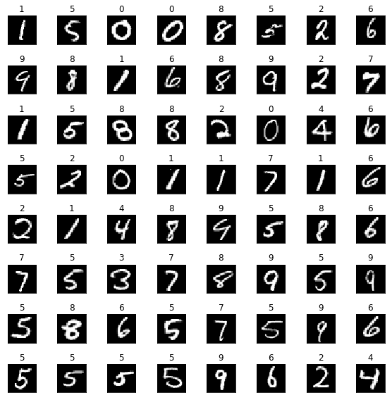
We will visualize a few of the MNIST images with their labels to get a feeling of how are training problem looks. Each drawn digit has it’s label on top.
images, labels = next(iter(train_loader))
fig, axes = plt.subplots(nrows=8, ncols=8)
for i, (image, label) in enumerate(zip(images, labels)):
    if i >= 64:
        break
    axes[i // 8][i % 8].imshow(images[i][0], cmap='gray')
    axes[i // 8][i % 8].set_title(f"{label}")
    axes[i // 8][i % 8].set_xticks([])
    axes[i // 8][i % 8].set_yticks([])
fig.set_size_inches(8, 8)
fig.tight_layout()
Below, we present a fully connected neural network to recognize the MNIST digits based on the architecture from the Dropout paper. The input to the network is the $28 \times 28$ MNIST grey-scale images flattened into a $784$-dimensional real-valued vector. The output is a vector representing the logarithm of the probability distribution over the 10 possible digit classes (0-9). We have three hidden layers (with bias), each containing 1024 neurons with dropout.
Formally, recall that we can see a neural network layer as a combination of a linear transformation $\mathbf{Z} = \mathbf{X}\mathbf{W}$ (where $X$ is the input and $W$ are the weights) and a non-linear operation $\mathbf{Y} = \eta(\mathbf{Z})$, where $\eta$ is a non-linear activation function (like sigmoid, hyperbolic tangent, ReLU, etc.). In our case, we use Leaky ReLU as non-activation function for hidden layers which simply keeps the value $y_i = z_i$ if it is non-negative ($z_i \geq 0$) and otherwise multiplies it with a small constant $y_i = z_i \times \delta$ (where $\delta$ is $10^{-2}$ per default). For the output-layer we apply the log-softmax function ($\tilde{y}_i = \log(\exp{z_i} / \sum_i \exp{z_i})$) to get a log-probability distribution (“logits”) of the output digits.
The core idea of dropout is to randomly drop a subset of neurons to improve generalization performance of the neural network. The percentage $p$ of neurons to drop is specified by the user, and in our case we set the probability of dropping a neuron to be $20\%$ for the input layer, and $50\%$ for the rest of the hidden layers (like the dropout paper). We can see dropout as a matrix $\mathbf{D}$ where each element is drawn from a probability distribution, $d_{ji} \sim \text{Bernoulli}(p)$, so $d_{ji}$ is $1$ with probability $p$ and otherwise $0$. The dropout matrix is element-wise multiplied to the weight vector before transforming the input, so $\mathbf{Z} = \mathbf{X}(\mathbf{W} \ast \mathbf{D})$.
class FCN(nn.Module):
    def __init__(self, n_classes=10):
        super(FCN, self).__init__()
        self.fc = nn.Sequential(nn.Dropout(p=0.2),
                                nn.Linear(784, 1024),
                                nn.Dropout(p=0.5),
                                nn.LeakyReLU(),
                                nn.Linear(1024, 1024),
                                nn.Dropout(p=0.5),
                                nn.LeakyReLU(),
                                nn.Linear(1024, 1024),
                                nn.Dropout(p=0.5),
                                nn.LeakyReLU(),
                                nn.Linear(1024, n_classes),
                                nn.LogSoftmax(dim=-1))

    def forward(self, inp):
        return self.fc(inp)

fcn = FCN()
We train the neural network using standard stochasic gradient descent, with a learning rate is $0.1$ and momentum $0.95$. We train for 30 epochs to see that the neural networks works, and gets a reasonable error rate.
We use the logits-based binary cross-entropy as a loss function so $\ell = - \sum_i y_i \log \tilde{p}_i$ where $\vec{y}$ is a 10-dimensional 1-hot encoding of target label (where $y_i = 1$ for label $i$ and all other elements are $0$) and $\log \tilde{p}_i$ are the predicted logits. We also print the accuracy of the network, which specifies how many percent of the labels in the training set, our network predicted correctly.
optim = SGD(fcn.parameters(recurse=True), lr=0.1, momentum=0.95)
for i in range(50):
    total_loss = 0.0
    total = 0.0
    correct = 0.0
    for images, labels in train_loader:
        fcn.zero_grad()
        pred = fcn.forward(images.cuda().view(-1, 784))
        loss = nnf.binary_cross_entropy_with_logits(pred, nnf.one_hot(labels.cuda(), 10).float())
        total_loss += loss
        total += labels.size(0)
        correct += (pred.argmax(-1) == labels.cuda()).sum().item()
        loss.backward()
        optim.step()
    print(f"[Epoch {i + 1}] loss: {total_loss:.5f} accuracy: {correct / total * 100:.5f}")
[Epoch 1] loss: 70.00793 accuracy: 67.70600
[Epoch 2] loss: 39.08666 accuracy: 91.61600
[Epoch 3] loss: 35.96854 accuracy: 93.79800
[Epoch 4] loss: 34.37635 accuracy: 94.83800
[Epoch 5] loss: 33.33277 accuracy: 95.57800
[Epoch 6] loss: 32.72926 accuracy: 95.98600
[Epoch 7] loss: 32.27712 accuracy: 96.34400
[Epoch 8] loss: 31.99868 accuracy: 96.44000
[Epoch 9] loss: 31.60433 accuracy: 96.76400
[Epoch 10] loss: 31.18402 accuracy: 97.03800
[Epoch 11] loss: 31.20170 accuracy: 97.04600
[Epoch 12] loss: 30.86907 accuracy: 97.31600
[Epoch 13] loss: 30.76726 accuracy: 97.39200
[Epoch 14] loss: 30.51833 accuracy: 97.46600
[Epoch 15] loss: 30.37416 accuracy: 97.64200
[Epoch 16] loss: 30.22861 accuracy: 97.73600
[Epoch 17] loss: 30.07159 accuracy: 97.83600
[Epoch 18] loss: 30.11995 accuracy: 97.84400
[Epoch 19] loss: 29.94004 accuracy: 97.94000
[Epoch 20] loss: 29.89834 accuracy: 97.95800
[Epoch 21] loss: 29.88626 accuracy: 97.93600
[Epoch 22] loss: 29.72416 accuracy: 98.08600
[Epoch 23] loss: 29.52944 accuracy: 98.19800
[Epoch 24] loss: 29.60426 accuracy: 98.11800
[Epoch 25] loss: 29.46951 accuracy: 98.30200
[Epoch 26] loss: 29.58494 accuracy: 98.16600
[Epoch 27] loss: 29.46461 accuracy: 98.31000
[Epoch 28] loss: 29.24048 accuracy: 98.43800
[Epoch 29] loss: 29.25820 accuracy: 98.32000
[Epoch 30] loss: 29.25681 accuracy: 98.35000
[Epoch 31] loss: 29.16539 accuracy: 98.45200
[Epoch 32] loss: 29.20642 accuracy: 98.40400
[Epoch 33] loss: 29.06911 accuracy: 98.48800
[Epoch 34] loss: 29.08886 accuracy: 98.56000
[Epoch 35] loss: 29.10168 accuracy: 98.52800
[Epoch 36] loss: 28.94155 accuracy: 98.58800
[Epoch 37] loss: 29.02398 accuracy: 98.63400
[Epoch 38] loss: 28.94587 accuracy: 98.58000
[Epoch 39] loss: 28.89379 accuracy: 98.67200
[Epoch 40] loss: 28.91088 accuracy: 98.60400
[Epoch 41] loss: 28.87774 accuracy: 98.68600
[Epoch 42] loss: 28.83196 accuracy: 98.74200
[Epoch 43] loss: 28.85329 accuracy: 98.69800
[Epoch 44] loss: 28.77813 accuracy: 98.74000
[Epoch 45] loss: 28.74476 accuracy: 98.74800
[Epoch 46] loss: 28.66849 accuracy: 98.78800
[Epoch 47] loss: 28.71410 accuracy: 98.77800
[Epoch 48] loss: 28.70339 accuracy: 98.85600
[Epoch 49] loss: 28.64754 accuracy: 98.80000
[Epoch 50] loss: 28.57953 accuracy: 98.83000
We evaluate our neural network on the test set and see that we also have a reasonable out-of-train performance.
total = 0.0
correct = 0.0
for images, labels in test_loader:
    pred = fcn.forward(images.cuda().view(-1, 784))
    total += labels.size(0)
    correct += (pred.argmax(-1) == labels.cuda()).sum().item()
print(f"Test accuracy: {correct / total * 100:.5f}")
Test accuracy: 97.14000
Bayesian Neural Networks
In the classical neural network, the weight matrix $\mathbf{W}$ for each layer was treated as a fixed-valued parameter to be optimized. In Bayesian neural networks, we would like to treat $\mathbf{W}$ as a random variable drawn from a probability distribution. A usual prior assumption is that each element in the weight matrix is drawn independently and identically from the standard normal distribution $w_{ji} \overset{\text{iid}}{\sim}\mathcal{N}(0, 1)$. Given some concrete input $\mathbf{X}$ and target predictions $\mathbf{Y}$, our goal is then to perform Bayesian inference where we want to learn a distribution of the weights that is adjusted to the given observed input and prediction values. In particular, for each layer we would like to learn a posterior over the weights $p(\mathbf{W} | \mathbf{X}, \mathbf{Y}) \propto p(\mathbf{Y} | \mathbf{X}, \mathbf{W}) p(\mathbf{W}) p(\mathbf{X})$ from the likelihood of labels given data $p(\mathbf{Y} | \mathbf{X}, \mathbf{W})$ and prior assumptions over weights $p(\mathbf{W})$ and data $p(\mathbf{X})$.
In practice, exact inference of the posterior distribution $p(\mathbf{W} | \mathbf{X}, \mathbf{Y})$ is analytically and computationally infeasible due to the involvement of so-called “intractable integrals” in the hidden normalization constant. An intractable integral is one which either cannot be solved analytically or where numeric integration is infeasible due to high-dimensional variables. In practice, we need to do approximation of the posterior distribution, and one way is to perform Variational Inference (VI). In Variational Inference, a closed-form parametric distribution $q_{\boldsymbol{\lambda}}(\mathbf{W})$ with optimizable parameters $\boldsymbol{\lambda}$ and then try to minimize the asymmetric Kullback-Leibler distance (divergence) to the true posterior $D_{\text{KL}}(q \parallel p)$. The posterior approximating distribution family $q$ is also called the guide, and is in the case of Bayesian NNs defined over the weights independently drawn from a normal distribution $w_{ji} \overset{\text{id}}{\sim} \mathcal{N}(\mu_{ji}, \sigma_{ji}^2)$, where $\mu_{ji}$ and $\sigma_{ji}$ are optimizable parameters representing the mean and standard deviation of each weight component in the layer. This guide is imprecise since it does not capture correlations between individual weights, but is feasible and reasonably fast to compute with.
Reparametrization
Sampling the weights from a non-standard normal distribution $w_{ji} \overset{\text{id}}{\sim} \mathcal{N}(\mu_{ji}, \sigma_{ji}^2)$ can introduce a lot of variance in the estimation of the KL divergence (because of large changes in the sampled values) which makes optimization hard. One trick to reduce variance is to use reparametrized sampling, where we perform sampling from the standard normal distribution $\varepsilon_{ji} \overset{\text{iid}}{\sim} \mathcal{N}(0, 1)$ and then use a deterministic transformation to compute the weights: $w_{ji} = \mu_{ji} + \sigma_{ji}\varepsilon_{ji}$.
For anything but small layers, we would still however need to sample many values which is computationally expensive. For example, if we have a layer with input and output dimensions $1000$, our weight matrix would have $1000\times1000 = 1 \text{ mio}$ elements, which must be sampled for each input value. The core idea of the local reparametrization trick is to instead sample the pre-activation values instead $\mathbf{Z} = \mathbf{X}\mathbf{W}$. This is done using a reparametrized transformation $z_i = \nu_i + \varsigma_i \epsilon_i$ with sampled normal distributed values like before $\epsilon_i \overset{\text{iid}}{\sim} \mathcal{N}(0, 1)$ and two deterministic computations over our parameters and inputs: \(\nu_i = \sum_j x_j \mu_{ji}\) and \(\varsigma_i^2 = \sum_j x_j^2 \sigma_{ji}^2\). Since our pre-activate values only depend on samples $\epsilon_i$ with index $i$ (not $j$), we get few orders of magnitudes savings in how much we need to sample. For the $1000\times1000$ weight example, we would only need to sample $1000$ values instead of $1 \text{ mio}$. This makes inference much more computationally feasible than before and allows scaling to much deeper networks.
Implementation in Pyro
We rely on Pyro’s implementation of Bayesian neural networks to implement a Bayesian version of the MNIST classifier. The architecture structure is the same as the classical network, except that the weights are sampled from a normal distribution instead of fixed and we use Leaky ReLU as non-linearity.
The main statement statement for specifying
sampling of value in Pyro is pyro.sample(name, dist), which takes a variable name name
and distribution to sample from dist as arguments. Our model uses this functionality
to sample from the HiddenLayer distribution from Pyro which implements local reparametrized sampling
of Bayesian neural network layers. The model uses standard normal as parameters a<n>_mean = 0.0 and
a<n>_scale = 1.0 with variational dropout ($\alpha = p / (1 - p)$) a<n>_dropout for each
non-output hidden layer (initialized so p is similar to the classical MNIST network).
We use the OneHotCategorical distribution to condition on our one-hot encoded labels (when provided)
using the obs keyword for the pyro.sample statement to do constraint the model to learn from the observed labels.
This is equivalent to specifying a binary cross-entropy loss as we did in the classical network.
The guide to approximate the posterior, sets up the parameters to be optimized using pyro.param,
making sure to provide reasonable initialization for the values and constraint them to relevant ranges.
It must sample the same latent (un-observed) variables as the model, although not necessarily from the same distribution.
To perform inference, we use the SGD optimizer with Nesterov momentum to minimize the KL divergence
which is calculated analytically for this model using the TraceMeanField_ELBO estimator. Pyro also supports a
wide variety of estimators to approximate the KL divergence, when it is not possible to calculate analytically
as in this case.
Finally, we perform an iterative optimization loop for a specified number of epochs to find the optimal
value of parameters, exactly like in the classical neural network model.
class BNN(nn.Module):
    def __init__(self, n_hidden=1024, n_classes=10):
        super(BNN, self).__init__()
        self.n_hidden = n_hidden
        self.n_classes = n_classes

    def model(self, images, labels=None, kl_factor=1.0):
        images = images.view(-1, 784)
        n_images = images.size(0)
        # Set-up parameters for the distribution of weights for each layer `a<n>`
        a1_mean = torch.zeros(784, self.n_hidden)
        a1_scale = torch.ones(784, self.n_hidden)
        a1_dropout = torch.tensor(0.25)
        a2_mean = torch.zeros(self.n_hidden + 1, self.n_hidden)
        a2_scale = torch.ones(self.n_hidden + 1, self.n_hidden)
        a2_dropout = torch.tensor(1.0)
        a3_mean = torch.zeros(self.n_hidden + 1, self.n_hidden)
        a3_scale = torch.ones(self.n_hidden + 1, self.n_hidden)
        a3_dropout = torch.tensor(1.0)
        a4_mean = torch.zeros(self.n_hidden + 1, self.n_classes)
        a4_scale = torch.ones(self.n_hidden + 1, self.n_classes)
        # Mark batched calculations to be conditionally independent given parameters using `plate`
        with pyro.plate('data', size=n_images):
            # Sample first hidden layer
            h1 = pyro.sample('h1', bnn.HiddenLayer(images, a1_mean, a1_dropout * a1_scale,
                                                   non_linearity=nnf.leaky_relu,
                                                   KL_factor=kl_factor))
            # Sample second hidden layer
            h2 = pyro.sample('h2', bnn.HiddenLayer(h1, a2_mean, a2_dropout * a2_scale,
                                                   non_linearity=nnf.leaky_relu,
                                                   KL_factor=kl_factor))
            # Sample third hidden layer
            h3 = pyro.sample('h3', bnn.HiddenLayer(h2, a3_mean, a3_dropout * a3_scale,
                                                   non_linearity=nnf.leaky_relu,
                                                   KL_factor=kl_factor))
            # Sample output logits
            logits = pyro.sample('logits', bnn.HiddenLayer(h3, a4_mean, a4_scale,
                                                           non_linearity=lambda x: nnf.log_softmax(x, dim=-1),
                                                           KL_factor=kl_factor,
                                                           include_hidden_bias=False))
            # One-hot encode labels
            labels = nnf.one_hot(labels) if labels is not None else None
            # Condition on observed labels, so it calculates the log-likehood loss when training using VI
            return pyro.sample('label', dist.OneHotCategorical(logits=logits), obs=labels)

    def guide(self, images, labels=None, kl_factor=1.0):
        images = images.view(-1, 784)
        n_images = images.size(0)
        # Set-up parameters to be optimized to approximate the true posterior
        # Mean parameters are randomly initialized to small values around 0, and scale parameters
        # are initialized to be 0.1 to be closer to the expected posterior value which we assume is stronger than
        # the prior scale of 1.
        # Scale parameters must be positive, so we constraint them to be larger than some epsilon value (0.01).
        # Variational dropout are initialized as in the prior model, and constrained to be between 0.1 and 1 (so dropout
        # rate is between 0.1 and 0.5) as suggested in the local reparametrization paper
        a1_mean = pyro.param('a1_mean', 0.01 * torch.randn(784, self.n_hidden))
        a1_scale = pyro.param('a1_scale', 0.1 * torch.ones(784, self.n_hidden),
                              constraint=constraints.greater_than(0.01))
        a1_dropout = pyro.param('a1_dropout', torch.tensor(0.25),
                                constraint=constraints.interval(0.1, 1.0))
        a2_mean = pyro.param('a2_mean', 0.01 * torch.randn(self.n_hidden + 1, self.n_hidden))
        a2_scale = pyro.param('a2_scale', 0.1 * torch.ones(self.n_hidden + 1, self.n_hidden),
                              constraint=constraints.greater_than(0.01))
        a2_dropout = pyro.param('a2_dropout', torch.tensor(1.0),
                                constraint=constraints.interval(0.1, 1.0))
        a3_mean = pyro.param('a3_mean', 0.01 * torch.randn(self.n_hidden + 1, self.n_hidden))
        a3_scale = pyro.param('a3_scale', 0.1 * torch.ones(self.n_hidden + 1, self.n_hidden),
                              constraint=constraints.greater_than(0.01))
        a3_dropout = pyro.param('a3_dropout', torch.tensor(1.0),
                                constraint=constraints.interval(0.1, 1.0))
        a4_mean = pyro.param('a4_mean', 0.01 * torch.randn(self.n_hidden + 1, self.n_classes))
        a4_scale = pyro.param('a4_scale', 0.1 * torch.ones(self.n_hidden + 1, self.n_classes),
                              constraint=constraints.greater_than(0.01))
        # Sample latent values using the variational parameters that are set-up above.
        # Notice how there is no conditioning on labels in the guide!
        with pyro.plate('data', size=n_images):
            h1 = pyro.sample('h1', bnn.HiddenLayer(images, a1_mean, a1_dropout * a1_scale,
                                                   non_linearity=nnf.leaky_relu,
                                                   KL_factor=kl_factor))
            h2 = pyro.sample('h2', bnn.HiddenLayer(h1, a2_mean, a2_dropout * a2_scale,
                                                   non_linearity=nnf.leaky_relu,
                                                   KL_factor=kl_factor))
            h3 = pyro.sample('h3', bnn.HiddenLayer(h2, a3_mean, a3_dropout * a3_scale,
                                                   non_linearity=nnf.leaky_relu,
                                                   KL_factor=kl_factor))
            logits = pyro.sample('logits', bnn.HiddenLayer(h3, a4_mean, a4_scale,
                                                           non_linearity=lambda x: nnf.log_softmax(x, dim=-1),
                                                           KL_factor=kl_factor,
                                                           include_hidden_bias=False))

    def infer_parameters(self, loader, lr=0.01, momentum=0.9,
                         num_epochs=30):
        optim = pyroopt.SGD({'lr': lr, 'momentum': momentum, 'nesterov': True})
        elbo = TraceMeanField_ELBO()
        svi = SVI(self.model, self.guide, optim, elbo)
        kl_factor = loader.batch_size / len(loader.dataset)
        for i in range(num_epochs):
            total_loss = 0.0
            total = 0.0
            correct = 0.0
            for images, labels in loader:
                loss = svi.step(images.cuda(), labels.cuda(), kl_factor=kl_factor)
                pred = self.forward(images.cuda(), n_samples=1).mean(0)
                total_loss += loss / len(loader.dataset)
                total += labels.size(0)
                correct += (pred.argmax(-1) == labels.cuda()).sum().item()
                param_store = pyro.get_param_store()
            print(f"[Epoch {i + 1}] loss: {total_loss:.5E} accuracy: {correct / total * 100:.5f}")

    def forward(self, images, n_samples=10):
        res = []
        for i in range(n_samples):
            t = poutine.trace(self.guide).get_trace(images)
            res.append(t.nodes['logits']['value'])
        return torch.stack(res, dim=0)
pyro.clear_param_store()
bayesnn = BNN()
bayesnn.infer_parameters(train_loader, num_epochs=30, lr=0.002)
[Epoch 1] loss: -1.05283E+02 accuracy: 29.95000
[Epoch 2] loss: -1.07710E+02 accuracy: 90.20200
[Epoch 3] loss: -1.08828E+02 accuracy: 94.39800
[Epoch 4] loss: -1.09825E+02 accuracy: 95.93200
[Epoch 5] loss: -1.10787E+02 accuracy: 96.70400
[Epoch 6] loss: -1.11732E+02 accuracy: 97.14000
[Epoch 7] loss: -1.12672E+02 accuracy: 97.55800
[Epoch 8] loss: -1.13607E+02 accuracy: 97.90400
[Epoch 9] loss: -1.14533E+02 accuracy: 98.18600
[Epoch 10] loss: -1.15453E+02 accuracy: 98.38600
[Epoch 11] loss: -1.16371E+02 accuracy: 98.57200
[Epoch 12] loss: -1.17284E+02 accuracy: 98.81600
[Epoch 13] loss: -1.18193E+02 accuracy: 98.94200
[Epoch 14] loss: -1.19095E+02 accuracy: 99.05400
[Epoch 15] loss: -1.19993E+02 accuracy: 99.14000
[Epoch 16] loss: -1.20890E+02 accuracy: 99.27600
[Epoch 17] loss: -1.21780E+02 accuracy: 99.39000
[Epoch 18] loss: -1.22660E+02 accuracy: 99.35400
[Epoch 19] loss: -1.23546E+02 accuracy: 99.48000
[Epoch 20] loss: -1.24430E+02 accuracy: 99.61200
[Epoch 21] loss: -1.25295E+02 accuracy: 99.61000
[Epoch 22] loss: -1.26169E+02 accuracy: 99.62800
[Epoch 23] loss: -1.27036E+02 accuracy: 99.70600
[Epoch 24] loss: -1.27896E+02 accuracy: 99.72000
[Epoch 25] loss: -1.28755E+02 accuracy: 99.75000
[Epoch 26] loss: -1.29607E+02 accuracy: 99.76400
[Epoch 27] loss: -1.30460E+02 accuracy: 99.82800
[Epoch 28] loss: -1.31301E+02 accuracy: 99.80600
[Epoch 29] loss: -1.32142E+02 accuracy: 99.81800
[Epoch 30] loss: -1.32980E+02 accuracy: 99.80600
total = 0.0
correct = 0.0
for images, labels in test_loader:
    pred = bayesnn.forward(images.cuda().view(-1, 784), n_samples=1)
    total += labels.size(0)
    correct += (pred.argmax(-1) == labels.cuda()).sum().item()
print(f"Test accuracy: {correct / total * 100:.5f}")
Test accuracy: 96.92000
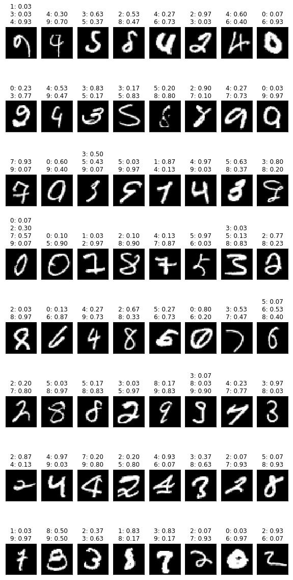
We now show how the neural network can be uncertain about its predictions
uncertain_images = []
for image, _ in test_loader:
    n_samples = 30
    preds = bayesnn.forward(image.cuda().view(-1, 784), n_samples=n_samples).argmax(-1).squeeze()
    pred_sum = [(i, c) for i, c in enumerate(preds.bincount(minlength=10).tolist()) if c > 0]
    if len(pred_sum) > 1:
        uncertain_images.append((image, "\n".join(f"{i}: {c / n_samples:.2f}" for i, c in pred_sum)))
    if len(uncertain_images) >= 64:
        break
fig, axes = plt.subplots(nrows=8, ncols=8)
fig.subplots_adjust(hspace=2.0)
for i, (image, label) in enumerate(uncertain_images):
    axes[i // 8][i % 8].imshow(image[0][0], cmap='gray')
    axes[i // 8][i % 8].set_title(f"{label}")
    axes[i // 8][i % 8].set_xticks([])
    axes[i // 8][i % 8].set_yticks([])
fig.set_size_inches(8, 16)
fig.tight_layout()